Part 1. Analysis-methods case-study – climate change at Gladstone
A science critique by Dr. Bill Johnston, Former research scientist, NSW Department of Natural Resources.
Dr. Bill Johnston’s scientific interests include agronomy, soil science, hydrology and climatology. With colleagues, he undertook daily weather observations from 1971 to about 1980.
Main points
- Gladstone Radar is used to case study an objective method of analysing trend and changes in temperature data. The 3-stage approach combines step-change and covariance analysis to resolve site change and covariable effects simultaneously and is applicable across the Australian Bureau of Meteorology’s climate-monitoring network.
- Accounting for site and instrument changes leaves no residual trend or change in Gladstone’s climate.
1. Introduction and background
In this age of concocted fake-news it is vital to use unbiased methods to detect trends and changes in the climate. Essential requirements are that:
- The approach is physically based, transparent and statistically sound.
Provided the process is underpinned by accepted physical principles, alignment with those principles assesses soundness of the data.
- Methods are robust and replicable.
Robust methods ensure reanalysis of the same or similar datasets results in comparable outcomes. In-built checks ensure integrity of the approach.
- Study of particular datasets is not influenced by prior knowledge neither can analysis be gamed to achieve a desired result.
The approach is independent and unbiased and outcomes are attributed post hoc.
Part 1 of this 4-part series uses data for Gladstone Radar (Bureau ID 39326; 1958 to 2017) to case study application of energy balance principles to analysing temperature (T) datasets for Cairns, Townsville and Rockhampton, which are ACORN-SAT (http://www.bom.gov.au/climate/change/acorn-sat/documents/ACORN-SAT-Station-adjustment-summary.pdf) sites representative of the northern, central and southern sectors of the Great Barrier Reef and which contribute to calculating Australia’s warming.
The site in Happy Valley Park is located within the city of Gladstone approximately 500 km north of Brisbane at Radar Hill Lookout (Latitude 3.8553, Longitude 151.2628), which is west of the city centre and port facilities. Daily data downloaded from the Bureau’s climate data online facility were summarised into an annual dataset (Appendix 1).
According to site-summary metadata, observations commenced in November 1957; a Fielden automatic weather station (AWS) was installed in 1991; changes to the radar setup occurred in 1972 and 2004; the A-pan evaporimeter and manual thermometers were removed in 1993 (so manual observations ceased); a humidity probe installed in 1993 was replaced in 2002 and the temperature probe installed in 1991 was replaced in 2004. Aerial photographs (QAP5850056 (2002)) and Google Earth Pro satellite images show the met-office was demolished and replaced between 2003 and 2006 (Figure 1). Site diagrams show the Stevenson screen relocated between 2004 and 2005 but metadata does not mention when a 60-litre screen replaced the former 230-litre one or when the current Almos AWS commenced operating. Missing data from when thermometers were removed in 1993 to 2000 showed out-of-range values were culled and that the AWS was probably replaced in late 2000.
The question is whether trajectory of the data reflect site and instruments changes or changes in the climate.

Figure 1. The Gladstone Radar met-office on 17 May 2003 (left; portion of QAP5850057) and 4 January 2006 (Google Earth Pro satellite image). The Stevenson screen and AWS cabinet is visible in the satellite image. Images are comparably scaled and aligned. Trees up to 6 m surround the cleared area. The site was reconfigured when the office was demolished in 2004. (Note: Queensland aerial photographs (QAP) are accessible on line at: https://qimagery.information.qld.gov.au/ )
2. The physical basis
2.1 Maximum temperature
Consistent with the First Law of thermodynamics, evaporation cools the local environment by removing energy as latent heat at the rate of 2.45 MJ/kg of water evaporated, which at dryland sites can’t exceed the rainfall (± 5%; dewfall may not be measured for example, neither is runoff or drainage below the root zone).
As 1 mm rainfall = 1 kg/m2, evaporation of Gladstone Radar median rainfall (841 mm) accounts for 2060 MJ/m2/yr of available energy (the balance between incoming short-wave solar and long-wave radiation emitted to space), which is 27.6% of average solar exposure (7470 MJ/m2/yr) estimated by the Bureau since January 1990 using satellite and albedo data. Assuming that at annual timesteps cyclical gains and losses by the landscape (ground heat flux) cancel-out, remaining net energy, the proportion not used for evaporation, is advected to the local atmosphere as sensible heat, which is measured as maximum temperature (Tmax) by thermometers held 1.2 m above the ground in a Stevenson screen. Thus the First Law theorem predicts that dry years are warm and the drier it is the warmer it gets.
In the parlance of the statistical package R https://www.r-project.org/ ), for a consistent well maintained site, dependence of Tmax on rainfall (Tmax ~ rainfall) is likely to be statistically significant (PregZero <0.05) and explain more than 50% of Tmax variation (R2adj >0.05). However, if site control is poor or observations are lackadaisical, significances and variation explained is less and in the extreme case that Tmax is random to rainfall, data don’t reflect the weather and are not useful for tracking trends and changes in the climate. In keeping with the First Law theorem, statistical significances of coefficients and variation explained objectively characterise data fitness.
2.2 Minimum temperature
Minimum temperature (Tmin), which occurs in the early morning usually around dawn, measures the balance between heat stored by the landscape the previous day and heat lost by long-wave radiation to space overnight. Although affected by cloudiness/humidity, which reduces emissions, and local factors such as inversions and cool-air drainage, a statistically significant dependent relationship is expected between Tmin and Tmax.
To summarise, while rainfall (which also proxies cloudiness) directly reduces Tmax via the water cycle (Figure 2(a)), its relationship with Tmin may not be significant (Figure 2(b)). In contrast, the relationship between Tmin and Tmax (sometimes expressed as the diurnal temperature range (DTR)) is expected to be linear and robust (i.e. significant (PregZero <0.05) with more than >50% of Tmin variation explained) (Figure 2(c)).
For both Tmax and Tmin, poor site control (local changes and inconsistencies including poor maintenance, irregular watering etc.) and omitted variable bias (failing to account for a known systematic effect) are the two main factors affecting significance (P) and statistical precision (R2adj). In Figure 2, as rainfall explains just 7.2% of Tmax variation and Tmax only 37.7% of variation in Tmin, it is likely that other factors are unexplained by the naïve case.

Figure 2. Naïve relationships between Tmax and Tmin and rainfall, and Tmin and Tmax. Median rainfall and average Tmax and Tmin are indicated by dotted lines. Values that appear to be out of range relative to that year’s rainfall (or Tmax) are indicated. Tmin is not correlated with rainfall (PregZero >0.05).
3. Statistical methods
3.1 Stepwise analysis
As site and instrument changes occur in parallel with observations, trend and change is confounded within the overall signal. Stepwise analysis separates the confounded signal, tests for significant changes in the data and verifies they are associated with site changes. The aim is to provide an unbiased explanation of the process, which is the evolution of temperature through time.
Stages of the analysis are:
- Significance (PregZero) and strength (R2adj) of relationships between Tmax and Tmin and rainfall, and Tmin and Tmax is investigated using linear regression in the first instance (Figure 2). However, only relationships between T and statistically significant covariates are of interest (Figure 2(a) and Figure 2(c)).
Linear regression partitions overall variation in temperature into that attributable to the covariate (deterministic variation represented by the straight lines in Figure 2) and the residual component, which although expected to be random potentially embed site-change effects.
- Re-scaled by adding grand-mean T, randomness of residuals is evaluated using an objective statistical test of the hypothesis that mean-T is constant (i.e. that rescaled residuals are homogeneous).
Abrupt, step-changes or (Sh)ifts in re-scaled means that do not return to their previous level indicate the background heat-ambience of the site or something related to the instrument changed independently of the covariate. Detected step-changes are referenced where possible using metadata, historic site information and aerial photographs otherwise statistical inference is the only evidence that data are not homogeneous. (If residuals are random there are no inhomogeneities.)
- Step-change analysis is verified using multiple linear regression of the Tcovariate relationship with step-change scenarios specified as category variables (viz. T ~ Shfactor + covariate).
Possible outcomes are: (a), Shfactor means are the same and interaction ( The R function lm is used to fit linear models (i.e. estimate coefficients from data and evaluate the overall
model fit); Type II analysis of variance (car package) conducts hypothesis tests on coefficients; a separate test
(of the form Tmax ~ Shfactor * covariate) evaluates equality of regression slopes while lsmeans tests differences
between segment means controlling for the covariate. )
between Shfactor and the covariate is not significant [segments are coincident, in which case they are indexed the same and reanalysed]; (b), Shfactor means are different and interaction is not significant [segmented responses to the covariate is the same (i.e. lines are parallel) and the covariate-adjusted difference between segment means measures the ‘true’ magnitude of the discontinuity]; (c) interaction is significant [responses are not consistent; Shfactor specification is irrelevant or changepoints are redundant (Shfactor changepoints don’t reflect the data)]; (d), T is random to the covariate [observations are not consistent, don’t reflect the weather and can’t reflect the climate].
Multiple linear regression residuals (i.e. data minus significant Shfactors and covariate effects) are examined for normality, equality of variance across categories, independence (autocorrelation) and serial clustering. Trend of individual segments is checked to assure the step-change model is appropriate.
3.2 Statistical tools
Sequential t-test analysis of regime shifts (STARS https://pdfs.semanticscholar.org/7746/6a6af18275339c2ef0bf4959e1c20b3b82cd.pdf ) is used for step-change analysis of both raw-T and re-scaled residuals (https://www.beringclimate.noaa.gov/regimes/) and the R packages https://www.rcommander.com/; https://cran.r-project.org/web/packages/lsmeans/lsmeans.pdf) Rcmdr and lsmeans are used for linear and multiple linear regression and to test differences between segment means holding the covariate constant (at its median (rainfall) or average (Tmax) level). Additional tests (normality, independence, clustering, Kruskall-Wallis (non-parametric) 1-way analysis of variance on ranks) etc. are performed using the statistical application PAST from the Natural History Museum, University of Oslo (https://folk.uio.no/ohammer/past/). As data and statistical tools are in the public domain analyses is fully replicable.
3.3 Comparing change scenarios
Multiple linear regression is used to compare Shfactor scenarios, for instance that documented site changes (ShSite) are influential on T or if other changepoints better fit the data. While all combinations are evaluated, the disciplined outcome is that segmented regressions are offset and parallel (Section 3.1 (iii (b)). It’s possible for example, that the main site change was in 1991 when the AWS was installed; or in 1993, when manual observation ceased; or in 1993 and 2004 when the met-office was demolished (Figure 1). Alternatively, there was a Tmax step-change in 2004 and a Tmax rainfall-residual step-change in 2001 (which is not cross-referenced by available metadata but as it aligns with when missing observation ceased, the AWS was possibly replaced and a 60-litre Stevenson screen installed in place of the previous 230-litre one). Selected Tmax scenarios are shown in Figure 3.

Figure 3. Horizontal lines plausibly explain persistent changes in raw Tmax. With the exception of the 2001 shift in (d), which is detected statistically using STARS, segmented-means for each scenario are calculated manually as examples. Multiple linear regression tests if Tmax is correlated with rainfall overall and if differences in median-rainfall adjusted means are the same (indicated by letters beside each line). In all cases interaction is not significant (ns), which confirms that free-fit lines are statistically parallel.
The same site changes potentially affect Tmin. In addition, there is a shift in Tmin vs. Tmax-residuals in 1973, 1983 and 1999 (ShMinMaxRes) and first-round analysis found no difference in segment means from 1973 to 1982 and from 1999 to 2017 (thus segments are coincident). Another scenario results from combining those segments (ShMinMaxRes1). There is also a shift in raw-Tmin in 1979, which could reflect the weather or something else.
The experiment is run in reverse – data are available but the experimental design (the ‘treatments’ and when they were applied) is unknown. It is important the problem is approached without bias (i.e. all possibilities are on the table) and that analysis is independent and statistically disciplined (i.e. that covariate coefficients are significant, adjusted segment means are different indicating lines are offset and interaction is not significant).
So the question is: which scenario best explains each dataset?
Results of the scenario analysis are summarised in Table 1. For Tmax, the expected physical dependence of Tmax on rainfall is not significant (P >0.05) for scenarios (ii) and (iii), which indicates hypothesised step-changes are irrelevant (significance is reduced relative to (i), which is the base-case). Although the covariate is significant for scenario (iv) the hypothesised change in 1993 is not (rainfall adjusted segment means pre- and post-1993 (to 2003) are the same. Scenarios (v) and (vi) appear to be equivalent; however variation explained by Scenario (vi) is higher (51.7% vs. 43.4%), and the Akaike information criterion (AIC –
Burnham, K.P, Anderson, D.R and Huyvaert, K.P. 2011. AIC model selection and multimodel inference in
behavioral ecology: some background, observations, and comparisons. Behav Ecol Sociobiol 65, 23-35. doi
10.1007/s00265-010-1029-6) (which measures the relative quality of alternative models describing the same dataset) is lower, indicating Scenario (vi) is the better (more parsimonious) fit. (AIC is not given where factors and or the covariate are not significant.)
There is no other way to cut-and-dice the data consistent with the requirements that the covariate coefficient is significant and segmented regressions are parallel and offset by a difference that reflects the site-change response. Furthermore, Scenario (vi) regression residuals are normally distributed, independent (not autocorrelated), and their variance is the same across categories (residuals are homoscedastic). With those three assumptions satisfied, no additional systematic factors are influential on Tmax. There is also no residual trend.
The step-change in 2001 (0.83oC median-rainfall adjusted) is responsible for the raw-Tmax trend (0.16oC/decade; Punc <0.001) and as trend before and after the changepoint is not different to zero-trend, the step-change model best fits the data. Although when the met-office was demolished in 2004 year-to-year variability appeared to increase, suspected replacement of the AWS operating with a 60-litre screen in 2001 is the likely cause of the up-step.
Tmin first-round analysis (Tmin ~ Tmin-Tmax residuals + Tmax) found average-T for the segment from 1973 (corresponding with metrication on 1 September 1992) to 1982 (Figure 4 (a)) is the same as the segment from 1999 to 2017 (18.65oC (SE 0.080) vs 18.49 (0.065)). Although the slope of the first mentioned regression is skewed higher by data for 1973 and 1980 (Figure 4 (b); Table 1, Tmin Case (iv)), as segments are statistically coincident they combine into a single category (Table 1, Tmin Case (v)). Second-round analysis (Figure 4 (c)) shows regressions are parallel and offset; Tmin increases 0.59oC/oCTmax and with Tmax held at its long-term average (27.6oC) the cumulative Tmin difference from the start of the record is 0.28oC. Furthermore, multiple linear regression residuals and individual data segments in Figure 4 (a) are untrending. Although data for 1960, 1974, 1983 and 2010 are likely outliers (but not excluded), the overall raw-Tmin trend of 0.16oC/decade (Punc <0.001) is spuriously due to site and instrument changes not the climate.
Table 1. Multiple linear regression of Tmax and Tmin change scenarios. Non significance (ns) of the covariate indicates lack of agreement between the statistical model and the First Law theorem.
| Tmax vs. rainfall | Change yearsSignificance | Covariate (P) (R2adj) | AIC | Covariate coefficient |
| (i) Tmax ~Rainfall | na | 0.02 (0.072) | 100.43 | -0.060oC/100 mm rainfall |
| (ii) ShSite | 1991P <0.001 | 0.055 (ns) | ||
| (iii) ShSite1 | 1993P <0.001 | (ns) | ||
| (iv) ShSite2 | 1993ns & 2004 P <0.001 | 0.003 (0.486) | ||
| (v) ShMax | 2004 P =0.001 | 0.003 (0.434) | 71.70 | -0.069oC/100 mm rainfall |
| (vi) ShMaxRes | 2001 P <0.001 | <0.001 (0.517) | 62.16 | -0.057oC/100 mm rainfall |
| Tmin vs Tmax | ||||
| Tmin ~ Tmax | na | <0.001 (0.377) | 48.50 | 0.49oCmin/oCmax |
| (i) ShSite | 1991P <0.033 | <0.001 (0.415) | 45.70 | 0.39oCmin/oCmax |
| (ii) ShSite1 | 1993ns | <0.001 | 0.40oCmin/oCmax | |
| (iii) ShSite2 | 1993ns & 2004ns | <0.001 | 0.45oCmin/oCmax | |
| (iv) ShMinMxRes | 1973, 1983 & 1999 | <0.001 (0.695) | 0.59oCmin/oCmax; segment means 1973-82 and >1999 are the same. | |
| (v) ShMinMxRes1 | 1973, 1983 & 1999 | <0.001 (0.688) | 8.88 | 0.54oCmin/oCmax; comb. 1973-82 & >1999 |
| (vi) ShMinMxRes2 | 1973P <0.001 & 1999P <0.018 | <0.001 (0.661) | 13.92 | 0.59oCmin/oCmax |
| (vii) ShMin | 1979 | <0.001 (0.547) | 30.36 | 0.40oCmin/oCmax |
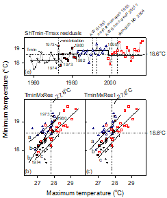
Figure 4. Step-changes in re-scaled Tmin-Tmax residuals detected by STARS are aligned with documented (and suspected) site and instrument changes post hoc (a). As step-changes cannot be specified in advance, STARS is a blind test of the null hypothesis that the cumulative rescaled residual mean is unchanged. The upstep in 1973 corresponds with the screen possibly moving out of the way of a new radar tower installed in May 1972 and also replacement of the Fahrenheit thermometers with Celsius ones from 1 September 1972. The 1982 changepoint could be due to the yard being extended other changes that happened between 1969 and 1992. Regression lines in (b) and (c) are free-fit.
4. Discussion
4.1 Metadata can’t be trusted
Analysis of climate time-series presumes no extraneous factors impact on data. Aerial photographs (Figure 5) show the yard behind the met-office was extended between 1969 and 1992 and the profile of the office also changed. It is likely the screen was moved out of the way when a 30-foot (10 m) radar tower was installed in May 1972 but other potentially influential changes are not listed in metadata. As some documented site changes don’t affect data and others that do may not be documented a robust independent changepoint detection method combined with post hoc research is an essential first step in assessing the fitness of temperature data for depicting trends and changes in the climate.

Figure 5. Aerial photographs show the met-office was enlarged and the area behind the building was cleared and expanded between November 1969 (left) and January 1992 (zoomed and cropped portions of QAP204702 and QAP502722). WF44 radar was installed in on a lattice tower in May 1972 but other changes and when they occurred are not detailed in site-summary metadata. (Photos are aligned at about the same scale.)
4.2 The statistical approach
The objective of the study was to outline a methodology for exploring trends and changes in Tmax and Tmin data in sufficient detail that the approach is replicable and can be applied to other datasets. If multiple linear regression fully explains changes and trends in raw data and it adequately reflects the data generating process, residuals are normally distributed, independent (individual values do not predict future values i.e. there is no autocorrelation), and variance is random (homoskedastic) across categories. Analysing raw temperature data in the time-domain (vs. the covariate-domain) is made difficult by confounding of site changes with observations. Furthermore, unless the covariate is also accounted for, apparent changes in T can be due to sustained shifts in the covariate say due to the El Niño southern oscillation effects on rainfall. Multiple linear regression removes covariate and step-change signals simultaneously, which provides an unbiased assessment of the data-generating process.
4.3 Site and instrument changes
For a warming argument to prevail claimants must adjust for all other possible sources of bias, including in Gladstone Radar’s case that site changes between 1969 and 1992 and 2003 and 2006; installation and upgrading of weather radars and changes to the AWS and Stevenson screens.
If an influential site or instrument change occurs, the baseline against which daily-T is measured shifts cooler or warmer depending on the nature of the change. A shift is a discontinuity in the data-stream that is independent of respective covariates – rainfall in the case of Tmax, antecedent T (Tmax) in the case of Tmin. Examining covariates using naïve linear regression (T ~ covariate) does not account for factors that reduce significances and goodness of fit (R2adj). These are detected (and attributed where possible using metadata and other sources) then fitted recursively as factors with the covariate as the independent variable. Comparing scenarios statistically, leads to a single parsimonious outcome.
Although unconfirmed by metadata, the abrupt Tmax step-change of 0.83oC in 2001, which is independent of rainfall, is suspected to be due to installation of the current Almos AWS operating with a 60-litre Stevenson screen in either 1999 or 2000. Site change effects in 1973, 1982 and 1999 caused Tmin to increase 0.28oC since 1958. Multiple linear regression assumptions are not violated so datasets are fully explained and as there is no residual trend, there is no evidence that the climate has changed or warmed.
5. Conclusions
The methodology outlined is robust and rigorous and has been used to analyse some 150 long and medium-term datasets from across Australia. The most prevalent problem: that poorly documented site and instrument changes create spurious trends and changes in naïvely analysed data, is circumvented by step-change analysis of T ~ covariate residuals together with multiple linear regression of Shfactor scenarios controlling for the covariable. Further, it is not possible to impose change-scenarios that are not relevant to the data without either infringing the First Law theorem that covariate coefficients are significant or the statistical outcomes that: (i), segmented regressions are parallel (interaction is not significant); (ii), slopes are offset by the true magnitude of the discontinuity (segmented means are different); and, (iii), that underlying statistical assumptions are not violated.
Finally, as multiple liner regression residuals embed no trend or step-changes there is no evidence that Gladstone’s climate has changed or warmed.
Appendix 1. Annual data for Gladstone Radar used in the study
| Year | Rain | MaxAv | MaxN | MaxVar | MinAv | MinN | MinVar |
| 1958 | 955 | 27.95699 | 365 | 13.64702 | 18.43315 | 365 | 14.20266 |
| 1959 | 791.4 | 27.34712 | 365 | 11.75717 | 18.06904 | 365 | 13.20006 |
| 1960 | 770.2 | 27.55492 | 366 | 16.10248 | 17.53115 | 366 | 17.32456 |
| 1961 | 1070 | 27.44396 | 364 | 11.74098 | 17.65962 | 364 | 12.58682 |
| 1962 | 1257.5 | 27.4589 | 365 | 13.10424 | 18.25123 | 365 | 12.67712 |
| 1963 | 813.8 | 27.16329 | 365 | 11.85804 | 18.01315 | 365 | 13.57444 |
| 1964 | 718.5 | 27.93962 | 366 | 15.13303 | 18.68333 | 366 | 14.25986 |
| 1965 | 432.5 | 27.74603 | 365 | 14.34441 | 18.15425 | 365 | 12.77963 |
| 1966 | 807.8 | 27.31315 | 365 | 14.60895 | 17.97123 | 365 | 13.33618 |
| 1967 | 770.2 | 27.60438 | 365 | 16.39004 | 18.01589 | 365 | 12.072 |
| 1968 | 1041.2 | 27.89399 | 366 | 18.59969 | 18.11284 | 366 | 16.82918 |
| 1969 | 842.3 | 28.12 | 365 | 17.63869 | 18.70904 | 365 | 13.81896 |
| 1970 | 839.6 | 28.3074 | 365 | 10.72481 | 18.4811 | 365 | 14.1467 |
| 1971 | 1731.6 | 27.29534 | 365 | 13.65023 | 18.22959 | 365 | 14.41786 |
| 1972 | 662.5 | 27.46913 | 366 | 10.93069 | 17.93798 | 366 | 12.80855 |
| 1973 | 1418.2 | 27.9825 | 360 | 11.98434 | 19.19917 | 360 | 11.11947 |
| 1974 | 1205.2 | 26.95562 | 365 | 11.69028 | 17.81918 | 365 | 15.9065 |
| 1975 | 988.2 | 27.29096 | 365 | 11.40945 | 18.61836 | 365 | 11.91315 |
| 1976 | 970.4 | 27.47705 | 366 | 14.2404 | 18.33579 | 366 | 16.77288 |
| 1977 | 967.2 | 27.15808 | 365 | 11.7586 | 18.2874 | 365 | 16.05319 |
| 1978 | 962.2 | 27.03945 | 365 | 17.0191 | 18.15589 | 365 | 16.65461 |
| 1979 | 527.2 | 27.91452 | 365 | 12.62559 | 18.66329 | 365 | 13.56524 |
| 1980 | 840.8 | 28.0224 | 366 | 12.3744 | 19.04235 | 366 | 13.49785 |
| 1981 | 972.8 | 27.47253 | 364 | 14.45781 | 18.41456 | 364 | 16.35712 |
| 1982 | 538.2 | 27.45068 | 365 | 13.98295 | 18.36548 | 365 | 16.63227 |
| 1983 | 1441.8 | 26.68904 | 365 | 12.33548 | 18.77151 | 365 | 13.80155 |
| 1984 | 544.2 | 27 | 366 | 12.79342 | 18.5235 | 366 | 13.71073 |
| 1985 | 782.6 | 27.21315 | 365 | 15.48466 | 18.64575 | 365 | 16.00133 |
| 1986 | 1040.4 | 27.29425 | 365 | 14.53477 | 18.83699 | 365 | 13.2569 |
| 1987 | 698.4 | 27.63014 | 365 | 14.19601 | 18.67288 | 365 | 14.45264 |
| 1988 | 1083.2 | 27.80656 | 366 | 13.74187 | 18.82541 | 366 | 11.40541 |
| 1989 | 1087.1 | 26.85918 | 365 | 15.57511 | 18.00411 | 365 | 17.03787 |
| 1990 | 983.8 | 27.47699 | 365 | 17.96167 | 18.55808 | 365 | 17.68596 |
| 1991 | 841.6 | 27.87342 | 365 | 9.507067 | 18.87753 | 365 | 13.8185 |
| 1992 | 1135.4 | 27.32131 | 366 | 15.3602 | 18.64563 | 366 | 15.9798 |
| 1993 | 469.6 | 27.92708 | 336 | 10.30538 | 19.30564 | 337 | 9.211248 |
| 1994 | 648.6 | 27.8274 | 354 | 11.85327 | 18.57017 | 352 | 13.22335 |
| 1995 | 539.6 | 27.86698 | 321 | 16.42016 | 18.99818 | 330 | 16.10863 |
| 1996 | 996 | 27.33528 | 360 | 14.34936 | 18.72674 | 359 | 14.56548 |
| 1997 | 630.2 | 27.48157 | 331 | 11.63199 | 18.93012 | 332 | 12.17776 |
| 1998 | 738.2 | 28.03015 | 335 | 14.69121 | 19.19304 | 345 | 14.5292 |
| 1999 | 842.6 | 27.18547 | 344 | 10.61658 | 18.31268 | 347 | 11.78666 |
| 2000 | 845.4 | 27.04944 | 360 | 11.49008 | 17.92033 | 364 | 12.61909 |
| 2001 | 442.2 | 28.28 | 360 | 11.6201 | 18.62527 | 364 | 13.31859 |
| 2002 | 577.2 | 28.38778 | 360 | 14.614 | 18.71644 | 365 | 14.1111 |
| 2003 | 1166.7 | 27.78788 | 363 | 9.807974 | 18.74093 | 364 | 11.1459 |
| 2004 | 698.2 | 28.70274 | 365 | 11.43675 | 18.87198 | 364 | 16.14428 |
| 2005 | 705.2 | 29.3074 | 365 | 15.64629 | 19.45726 | 365 | 14.4252 |
| 2006 | 663.4 | 28.80164 | 365 | 14.02203 | 18.83178 | 365 | 12.79717 |
| 2007 | 792.2 | 28.15644 | 365 | 17.56741 | 18.68301 | 365 | 16.12724 |
| 2008 | 1127 | 27.79342 | 365 | 14.17254 | 18.44027 | 365 | 15.56901 |
| 2009 | 650.4 | 29.08599 | 364 | 9.65647 | 19.08849 | 365 | 12.41602 |
| 2010 | 1559.6 | 27.48187 | 364 | 10.70165 | 18.88548 | 365 | 13.61729 |
| 2011 | 734.4 | 27.81397 | 365 | 13.7495 | 18.15014 | 365 | 16.94569 |
| 2012 | 764 | 27.8306 | 366 | 16.61281 | 18.37486 | 366 | 14.91668 |
| 2013 | 1446.4 | 28.33205 | 365 | 14.81114 | 18.94423 | 364 | 11.13608 |
| 2014 | 941.4 | 28.17088 | 364 | 12.137 | 18.82082 | 365 | 14.01753 |
| 2015 | 685.2 | 28.5843 | 363 | 12.7284 | 18.85234 | 363 | 14.2793 |
| 2016 | 951.6 | 28.60904 | 354 | 15.06949 | 19.39831 | 356 | 13.03081 |
| 2017 | 983.2 | 28.82473 | 364 | 10.41256 | 19.54278 | 360 | 12.27505 |